From Mean-Variance to the CAPM

In HW 0 you solved one investor’s portfolio problem. This page asks what happens when every investor solves it. The answer is the Capital Asset Pricing Model (CAPM), the theory behind the market index you build in HW 1. It gives statements and intuition only. Each step links to the paper where the result is proved. Along the way it names the four straight lines that textbooks draw for this theory, and a figure at the end puts them side by side.

The figures use ten well-known stocks from CRSP (Apple, Microsoft, Exxon, J&J, Walmart, Coca-Cola, JPMorgan, GE, Ford, and Disney), monthly from 1990 through 2024. They were picked with hindsight from among today’s best-known companies, so their average returns are higher than a typical stock’s. That does not matter for pictures about risk, but it means these figures are not a test of anything. The calculations are in src/calc_asset_pricing_theory.py.

Step 1: One investor holds the tangency portfolio

The tangency portfolio is the portfolio of risky assets with the highest Sharpe ratio. From HW 0, its weights are

\[ w_T \propto \Sigma^{-1}(\mu - r_f \mathbf{1}). \]

Statement (Tobin separation). When there is a risk-free asset, every mean-variance investor holds the same risky portfolio, the tangency portfolio. Risk aversion only decides how wealth is split between the tangency portfolio and the risk-free asset.

In symbols, with \(w_0^*\) the weight on the one risk-free asset (a scalar) and \(w^* = [\,w_1^*, \ldots, w_N^*\,]\) the weights on the \(N\) risky assets (a vector), the optimal portfolio is

\[ \underbrace{\big[\, w_0^*,\; w_1^*,\; \ldots,\; w_N^* \,\big]}_{\text{optimal portfolio}} \;=\; (1 - a)\,\underbrace{\big[\, 1,\; 0,\; \ldots,\; 0 \,\big]}_{\text{risk-free asset}} \;+\; a\,\underbrace{\big[\, 0,\; w_{T,1},\; \ldots,\; w_{T,N} \,\big]}_{\text{tangency portfolio}} . \]

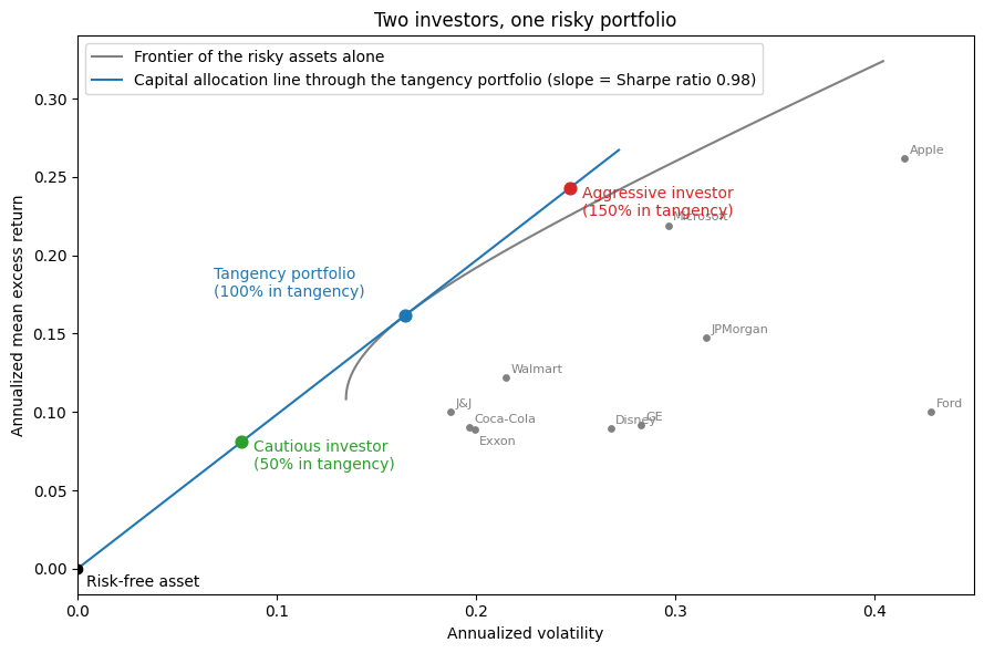
The first fund is the risk-free asset alone and the second is the tangency portfolio alone. Everyone holds the same \(w_T\). The one number that depends on the investor is the scalar \(a\), the share of wealth in the tangency portfolio: less than one for an investor who lends, more than one for one who borrows. The two investors in the figure have \(a\) equal to 0.5 and 1.5.

Intuition. Mixing the risk-free asset with a risky portfolio traces a straight line that starts at \(r_f\), and its slope is that portfolio’s Sharpe ratio. Each such line is a capital allocation line (CAL). Every investor wants the steepest one, whatever point on it they pick. A cautious investor lends part of their wealth at \(r_f\), and an aggressive one borrows to hold more than 100% in the tangency portfolio. Both hold the same mix of risky assets.

In the figure, the gray curve is the frontier of the ten stocks alone. The blue line is the steepest capital allocation line, the one from the risk-free asset that still touches the curve, and it touches at the tangency portfolio. The two investors sit on that line, one below the tangency point and one above.

Where \(a\) comes from. The statement above holds for any mean-variance investor without saying how risk aversion is measured. To put a number on it, take an investor with risk aversion \(\gamma\) who chooses the risky weights \(w\) to maximize \(E[R_p] - \tfrac{\gamma}{2}\,\mathrm{Var}(R_p)\), with the remainder \(w_0 = 1 - \mathbf{1}^\top w\) in the risk-free asset. Since \(E[R_p] = r_f + w^\top(\mu - r_f \mathbf{1})\) and \(\mathrm{Var}(R_p) = w^\top \Sigma w\), the first-order condition is

\[ w^* = \frac{1}{\gamma}\,\Sigma^{-1}(\mu - r_f \mathbf{1}), \]

the tangency vector scaled by a number. Risk aversion changes the length of \(w^*\), not its direction, and that is the separation. Given that, choosing \(a\) is the same problem with one risky asset, the tangency portfolio: maximize \(r_f + a(\mu_T - r_f) - \tfrac{\gamma}{2}\, a^2 \sigma_T^2\) over \(a\), where \(\mu_T\) and \(\sigma_T^2\) are the tangency portfolio’s expected return and variance. The solution is

\[ a = \frac{\mu_T - r_f}{\gamma\,\sigma_T^2}, \]

the tangency portfolio’s expected excess return per unit of its variance, divided by the investor’s risk aversion. So \(a\) falls as \(\gamma\) rises, and the figure’s cautious investor, with \(a\) of 0.5 against the aggressive investor’s 1.5, is 3 times as risk averse.

The HW 0 appendix proves the general two-fund theorem: without a risk-free asset, every frontier portfolio mixes the same two funds (Merton 1972). Tobin separation is the special case where one of the two funds is the risk-free asset. Paper: Tobin (1958).

Step 2: Two kinds of risk

In the Step 1 figure, every stock sits to the right of the capital allocation line. Take any one of them and slide it left, keeping its expected return, until it reaches the line. The point it lands on is a portfolio an investor can hold: a mix of the tangency portfolio and the risk-free asset. It has the stock’s expected return and less risk.

Definition. Measure along the horizontal line through the stock. The segment from the vertical axis to the capital allocation line is the stock’s systematic volatility. The segment from the line to the stock is the volatility that diversification removes.

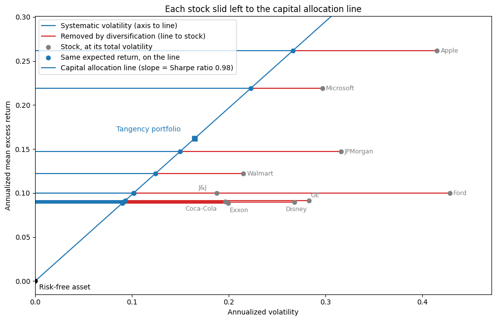
The systematic part is the part of the stock’s risk that moves with the tangency portfolio. If \(\rho_i\) is the stock’s correlation with the tangency portfolio, its systematic volatility is \(\rho_i \sigma_i\), and that is exactly where the stock lands on the line. This is algebra, not a finding. It holds for any set of assets and their own tangency portfolio, because the tangency weights are the ones at which every asset’s expected excess return is proportional to its covariance with the portfolio. Step 5 makes the same statement about the market, and there it can fail.

The rest of the stock’s risk is idiosyncratic: the part that does not move with the tangency portfolio. The two parts are uncorrelated, so their variances add,

\[ \sigma_i^2 = \underbrace{\rho_i^2 \sigma_i^2}_{\text{systematic}} + \underbrace{\sigma_{\varepsilon_i}^2}_{\text{idiosyncratic}} , \]

and the systematic share of the variance is \(\rho_i^2\). Volatilities do not add the same way. The two parts combine like the legs of a right triangle, with \(\sigma_i\) as the hypotenuse, so the idiosyncratic volatility \(\sigma_i \sqrt{1 - \rho_i^2}\) is longer than the red segment in the figure, \(\sigma_i (1 - \rho_i)\). The red segment is how much volatility the slide removes, not the volatility of what it removes. For Microsoft, the slide takes volatility from 30% to 22%, while its idiosyncratic volatility is 20%.

The figure uses the tangency portfolio of these ten stocks, and the split depends on that choice. The real frontier comes from optimizing over every risky asset. It would be a steeper line, and each stock would land at a different point on it. That portfolio cannot be estimated directly, because there are far more stocks than months of data. Step 4 argues that in equilibrium it is the market portfolio, and the example at the end of this page redoes the split against the market.

Statement (diversification). In a portfolio of many stocks, the idiosyncratic parts largely cancel and the systematic part remains. In an equal-weighted portfolio of \(N\) stocks, the idiosyncratic variance shrinks roughly like \(1/N\), and the systematic variance stays near the market’s.

Intuition. Firm-specific news is good for some firms and bad for others, so across many firms it averages out. Market-wide news hits all of them at once, so averaging cannot remove it.

The figure draws \(N\) stocks at random from every CRSP stock with a full return history since 1990, 200 times for each \(N\), and reports the average volatility of the equal-weighted portfolio. One stock has a volatility of 38% a year, ten have 20%, and a hundred have 16%, close to the market’s 15%. Past a few dozen stocks, adding more barely helps, because what is left is systematic risk. Paper: Evans and Archer (1968).

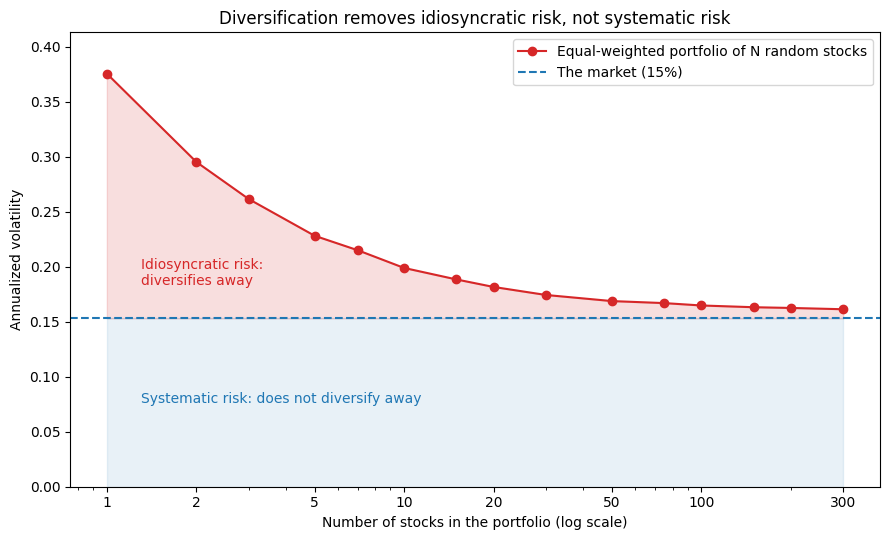
The slide in the first figure is diversification done optimally. For each level of expected return, mean-variance optimization sheds as much risk as can be shed. The random portfolios in the second figure shed most of it too, without optimizing anything.

Step 3: The assumptions

To go from one investor to a market, the CAPM assumes:

• Every investor is a mean-variance optimizer with a one-period horizon.

• Investors agree on \(\mu\) and \(\Sigma\) (homogeneous beliefs).

• Anyone can borrow or lend any amount at \(r_f\). There are no taxes or trading costs, and no investor is big enough to move prices.

• Risky assets are in positive net supply. They are the shares that exist, and their total value is the market capitalization.

• The risk-free asset is in zero net supply. It is a loan between investors, so every dollar lent is a dollar borrowed.

Step 4: Supply equals demand, so the market is the tangency portfolio

Statement. In equilibrium, the market portfolio, which holds every risky asset in proportion to its market value, is the tangency portfolio.

Intuition. By Step 1, every investor’s risky holdings are the same portfolio at different sizes. Add them up, and total demand for risky assets is the tangency portfolio, scaled up. Supply is the shares outstanding, which is the market portfolio. Prices adjust until demand equals supply, and at those prices the market is the tangency portfolio.

The figure shows a made-up economy with three stocks and three investors. Each investor’s stocks come in the same 50/30/20 mix; only the amount differs. The cautious investor lends $20, the aggressive investor borrows $20, and the moderate investor does neither. Add everyone up and the stocks are the market, while the risk-free positions sum to zero.

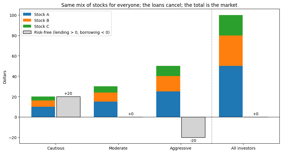
Because the risk-free asset is in zero net supply, borrowing and lending cancel. Investors as a whole hold none of it, and all wealth sits in the market portfolio. That fixes how large the market risk premium has to be: large enough that the average investor is willing to hold exactly the market, no more and no less.

\[ E[R_M] - r_f = \bar\gamma \, \sigma_M^2, \]

where \(\bar\gamma\) is investors’ average risk aversion. The premium is larger when investors are more risk averse or when the market is riskier.

The capital allocation line through the market portfolio has a name of its own, the capital market line (CML). Step 4 says that in equilibrium it is the steepest capital allocation line, the blue line of Step 1, because the market is the tangency portfolio.

Step 5: The CAPM

Statement (Sharpe 1964, Lintner 1965, Mossin 1966). Every asset’s expected excess return is proportional to its beta with the market:

\[ E[R_i] - r_f = \beta_i \big(E[R_M] - r_f\big), \qquad \beta_i = \frac{\mathrm{Cov}(R_i, R_M)}{\mathrm{Var}(R_M)}. \]

Intuition. Someone who holds the market cares only about the risk of the whole portfolio. An asset adds to that risk through its covariance with the market, not through its own variance. The rest of its risk, the idiosyncratic part, diversifies away, so it earns no reward. Because the market is already optimal, changing any asset’s weight cannot raise the Sharpe ratio. That only holds if every asset pays the same reward per unit of market risk it adds, and beta is that unit.

Only systematic risk is priced. Step 4 says the market is the tangency portfolio, so a stock’s systematic volatility is now measured against the market. With \(\rho_{iM}\) the stock’s correlation with the market, \(\rho_{iM} \sigma_i = \beta_i \sigma_M\), and the CAPM can be rewritten as

\[ E[R_i] - r_f = \underbrace{\frac{E[R_M] - r_f}{\sigma_M}}_{\text{market Sharpe ratio}} \times \underbrace{\beta_i \sigma_M}_{\text{systematic volatility}} . \]

Each unit of systematic volatility earns the market’s Sharpe ratio. Idiosyncratic volatility earns nothing.

Intuition. Anyone can get rid of idiosyncratic risk for free by holding a diversified portfolio, and in equilibrium everyone does, because they all hold the market. No one has to be paid to bear a risk they can shed for free. Systematic risk is different. It is the risk of the market portfolio itself, someone has to hold it, and so it has to be paid.

The figure is the Step 2 figure with the market in the tangency portfolio’s place. Each gray dot is a stock at its total volatility. The arrow moves it to its systematic volatility \(\beta_i \sigma_M\), the blue dot. The dashed line is the capital market line, from the risk-free asset through the market, and its slope is the market’s Sharpe ratio. In Step 2 the dots landed on the capital allocation line by construction. Here nothing forces them onto the capital market line. The CAPM is the claim that they land there: a stock’s reward depends on its systematic risk, however much total risk it has. Ford and Walmart illustrate this. Ford’s total volatility is 2.0 times Walmart’s, yet it earned less.

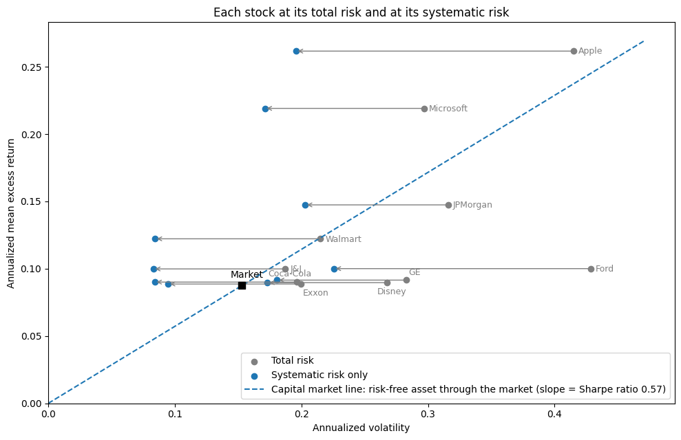
In these data, the blue dots do not land exactly on the line, and Apple and Microsoft are far above it. That gap is alpha, the subject of Step 6.

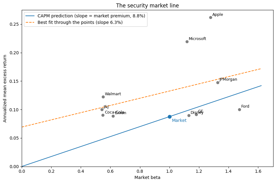
Plotted against beta, the CAPM is a straight line, the security market line (SML). It starts at zero (the risk-free asset has a beta of zero) and passes through the market at a beta of one. Its slope is the market risk premium. It is the figure above with beta, rather than \(\beta_i \sigma_M\), on the horizontal axis.

Step 6: What the CAPM predicts

Regress any portfolio’s excess return on the market’s excess return:

\[ R_{i,t} - r_{f,t} = \alpha_i + \beta_i (R_{M,t} - r_{f,t}) + \varepsilon_{i,t}. \]

This is the market model of Sharpe (1963). Its fitted line, one stock’s excess return against the market’s, is the stock’s security characteristic line (SCL). The slope is the stock’s beta and the intercept is its alpha.

The CAPM says \(\alpha_i = 0\) for every asset: every asset sits on the security market line, and its alpha is its vertical distance from the line. This is the same statement as “the market is the tangency portfolio.” A nonzero alpha means some mix of the market and portfolio \(i\) has a higher Sharpe ratio than the market alone (Gibbons, Ross, and Shanken 1989).

The figure plots the ten stocks. The blue line is what the CAPM predicts. The dashed line is the straight line that fits the stocks best.

An example: splitting risk in the data

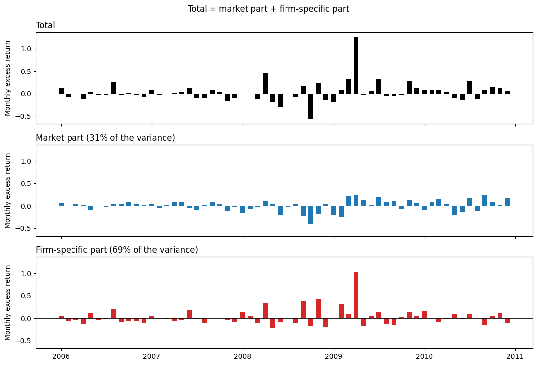
The regression in Step 6 also splits a stock’s return in two. The part \(\beta_i (R_{M,t} - r_{f,t})\) moves with the whole market. The rest, \(\varepsilon_{i,t}\), comes from news about the firm itself. The two parts are uncorrelated, so the variance splits as well:

\[ \sigma_i^2 = \underbrace{\beta_i^2 \sigma_M^2}_{\text{systematic}} + \underbrace{\sigma_{\varepsilon_i}^2}_{\text{idiosyncratic}} . \]

This is the Step 2 split with the market as the benchmark, since \(\beta_i \sigma_M = \rho_{iM} \sigma_i\). The shares change with the benchmark. Against their own tangency portfolio, the ten stocks’ systematic shares run from 6% (Ford) to 56% (Microsoft). A tangency portfolio fit in sample to ten stocks picked with hindsight is the extreme case: it shorts GE, Ford, and Disney, and it explains only 6% to 12% of their variance. Against the market, the shares below are more even.

The figure splits Ford’s monthly return from 2006 through 2010 into the two parts. The market part is mostly the 2008 crash, which hit every stock. The firm-specific part is Ford’s own story: the near-bankruptcy of the U.S. auto industry, then April 2009, when Ford rose 127% while its market part accounted for 25 points of that.

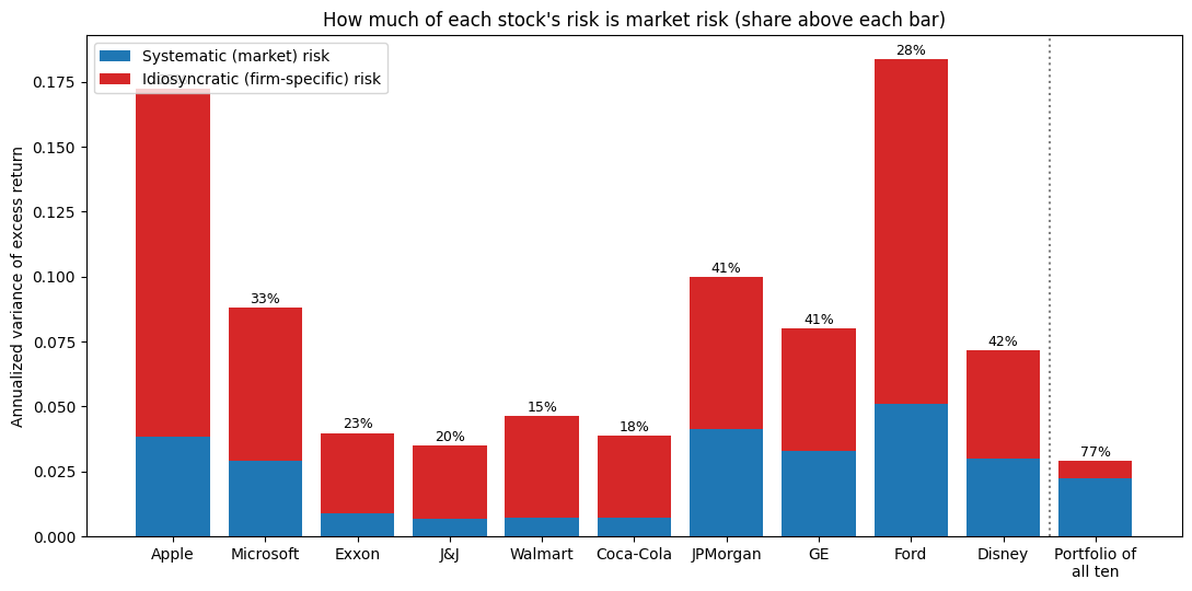
For most single stocks, idiosyncratic risk is most of the risk. For these ten, the market explains between 15% (Walmart) and 42% (Disney) of the variance. Put all ten in one equal-weighted portfolio, and the market explains 77%.

The four lines

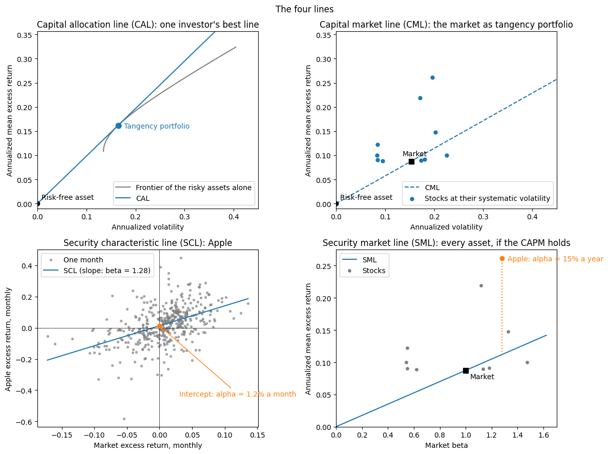
This page drew four straight lines that textbooks name. Two live in the volatility-return plane and two are built from beta. The figure puts them side by side, and the table says where each one came from. The layout follows a sketch by Graduate Tutor.

Line	Axes	What sits on it	Step
Capital allocation line (CAL)	volatility, expected return	mixes of the risk-free asset and one risky portfolio; the steepest CAL runs through the tangency portfolio	1
Capital market line (CML)	volatility, expected return	the CAL through the market portfolio; the same line as the steepest CAL if the market is the tangency portfolio	4
Security characteristic line (SCL)	market excess return, one stock’s excess return	the stock’s monthly returns, fitted; the slope is beta, the intercept is alpha	6
Security market line (SML)	beta, expected return	every asset, if the CAPM holds; a stock’s alpha is its vertical distance from the line	5

The lines come in two pairs. The first pair is the step from one investor to equilibrium: the capital market line is the capital allocation line once the market is the tangency portfolio. The second pair is the step from a time series to a cross-section: the security characteristic line is one stock’s history, and the security market line is the prediction for every stock. The same alpha appears in both. It is the intercept of the first, per month, and the vertical distance from the second, per year. Apple’s is marked in the figure.

In HW 1 you build the market index. Next week, HW 1 Guide E runs the alpha test on the portfolios your pipeline builds, and From the CAPM to Multifactor Models explains why more than one factor might be needed.

Discussion

The CAPM rests on the assumptions in Step 3. Which are hardest to believe, and what goes wrong when they fail?

Some answers that could come up:

• The market portfolio cannot be observed (Roll 1977). In theory it contains every risky asset: stocks, bonds, real estate, private businesses, even human capital. The CRSP value-weighted index is a stand-in. A test that rejects the CAPM may only show that the stand-in is not efficient, which is why Roll argues the theory cannot really be tested.

• Investors disagree. If beliefs differ, there is no single tangency portfolio for everyone to hold.

• Borrowing is neither free nor unlimited. Investors who cannot borrow get leverage by buying high-beta stocks instead, which pushes up their prices and flattens the relationship between beta and return (Black 1972; Frazzini and Pedersen 2014).

• The data agree. The relationship between average returns and beta is flatter than the CAPM predicts (Black, Jensen, and Scholes 1972; Fama and French 1992). The dashed line in the figure above is an example.

• One period. Real investors also care about what their opportunities will look like next year. Dropping this assumption leads to next week’s multifactor models.

• Mean and variance only. Investors may also care about skewness and crash risk, which is the subject of HW 3.

References

• Black, Fischer. “Capital Market Equilibrium with Restricted Borrowing.” Journal of Business 45, no. 3 (1972): 444-455.

• Black, Fischer, Michael C. Jensen, and Myron Scholes. “The Capital Asset Pricing Model: Some Empirical Tests.” In Studies in the Theory of Capital Markets, edited by Michael C. Jensen, 79-121. New York: Praeger, 1972.

• Evans, John L., and Stephen H. Archer. “Diversification and the Reduction of Dispersion: An Empirical Analysis.” Journal of Finance 23, no. 5 (1968): 761-767.

• Fama, Eugene F., and Kenneth R. French. “The Cross-Section of Expected Stock Returns.” Journal of Finance 47, no. 2 (1992): 427-465.

• Frazzini, Andrea, and Lasse Heje Pedersen. “Betting Against Beta.” Journal of Financial Economics 111, no. 1 (2014): 1-25.

• Gibbons, Michael R., Stephen A. Ross, and Jay Shanken. “A Test of the Efficiency of a Given Portfolio.” Econometrica 57, no. 5 (1989): 1121-1152.

• Lintner, John. “The Valuation of Risk Assets and the Selection of Risky Investments in Stock Portfolios and Capital Budgets.” Review of Economics and Statistics 47, no. 1 (1965): 13-37.

• Merton, Robert C. “An Analytic Derivation of the Efficient Portfolio Frontier.” Journal of Financial and Quantitative Analysis 7, no. 4 (1972): 1851-1872.

• Mossin, Jan. “Equilibrium in a Capital Asset Market.” Econometrica 34, no. 4 (1966): 768-783.

• Roll, Richard. “A Critique of the Asset Pricing Theory’s Tests Part I: On Past and Potential Testability of the Theory.” Journal of Financial Economics 4, no. 2 (1977): 129-176.

• Sharpe, William F. “A Simplified Model for Portfolio Analysis.” Management Science 9, no. 2 (1963): 277-293.

• Sharpe, William F. “Capital Asset Prices: A Theory of Market Equilibrium under Conditions of Risk.” Journal of Finance 19, no. 3 (1964): 425-442.

• Tobin, James. “Liquidity Preference as Behavior Towards Risk.” Review of Economic Studies 25, no. 2 (1958): 65-86.