From the CAPM to Multifactor Models

From Mean-Variance to the CAPM got the CAPM from one-period mean-variance investors and market clearing. This page drops the one-period assumption, and more than one factor appears. It then shows where Fama and French (1993) fit. As before, it gives statements and intuition only, with links to the papers that prove them.

The figures use Ken French’s 25 size and book-to-market portfolios and his three factors, monthly since 1965. The calculations are in src/calc_asset_pricing_theory.py.

Step 1: Why one period is not enough

The investment opportunities investors face change over time: interest rates move, expected returns rise and fall, and volatility comes and goes. An investor with a long horizon cares about next period’s wealth and about what that wealth will be able to earn afterward.

A state variable is anything that moves those future opportunities. The short rate, the market’s expected return, and market volatility are the usual examples. Collect the state variables in a vector \(X_t\), with \(K\) of them.

Step 2: The Intertemporal CAPM

The investor’s problem (Merton 1973). There are \(n\) risky assets and a risk-free asset, and investors can trade at every instant. Asset \(i\) has expected return \(\mu_i\), written \(E_t[R_i]\) below, and volatility \(\sigma_i\), and the risk-free rate is \(r_f\). None of the three is constant. They move with the state variables:

\[ \frac{dP_{i,t}}{P_{i,t}} = \mu_i(X_t)\,dt + \sigma_i(X_t)\,dz_{i,t}, \qquad dX_{k,t} = f_k(X_t)\,dt + g_k(X_t)\,dq_{k,t} . \]

Here \(dz_{i,t}\) and \(dq_{k,t}\) are the random shocks over the next instant. The investor chooses consumption \(c_t\) and portfolio weights \(w_t\) to maximize expected lifetime utility,

\[ \max_{\{c_t,\; w_t\}} \; E_0\!\left[\int_0^T U(c_t, t)\,dt + B(W_T, T)\right], \]

where wealth \(W_t\) grows with the portfolio’s return and shrinks with consumption:

\[ dW_t = W_t\left[\sum_{i=1}^n w_{i,t}\,\frac{dP_{i,t}}{P_{i,t}} + \Big(1 - \sum_{i=1}^n w_{i,t}\Big)\, r_f\,dt\right] - c_t\,dt . \]

\(U\) is the utility of consumption and \(B\) is the utility of the wealth left at the end. If \(\mu\), \(\sigma\) and \(r_f\) were constant, this investor would hold the tangency portfolio, as in the one-period problem. Because they move, the investor also cares how each asset’s return moves with \(X_t\).

Statement. The investor holds the tangency portfolio plus one hedging portfolio for each state variable, the portfolio of traded assets whose return moves most closely with changes in it. In equilibrium, with \(R_i\) the return on asset \(i\) over the next instant,

\[ E_t[R_i] - r_f = \beta_{i,M}\,\big(E_t[R_M] - r_f\big) + \sum_{k=1}^{K} \beta_{i,k}\,\big(E_t[R_{H_k}] - r_f\big), \]

where \(R_M\) is the return on the market and \(R_{H_k}\) is the return on the hedging portfolio for state variable \(k\). Merton (1973) derives this for one state variable, the interest rate. (The version with \(K\) state variables is in Merton 1992, Continuous-Time Finance, Section 15.10.) See either for the derivation.

Definition (the betas). These are the slopes in a regression of asset \(i\)’s excess return on all \(K+1\) portfolios at once:

\[ R_{i,t} - r_{f,t} = \alpha_i + \beta_{i,M}\,(R_{M,t} - r_{f,t}) + \sum_{k=1}^{K} \beta_{i,k}\,(R_{H_k,t} - r_{f,t}) + \varepsilon_{i,t} . \]

With no state variables, \(K = 0\), this is the market model of Step 6 in the CAPM reading, and the pricing equation above is the CAPM. With state variables, \(\beta_{i,M}\) is the market beta holding the hedging portfolios fixed, so it is generally not \(\mathrm{Cov}(R_i, R_M)/\mathrm{Var}(R_M)\). The ICAPM says \(\alpha_i = 0\) for every asset.

Intuition. An asset that pays off when opportunities get worse is insurance. Investors want it, bid up its price, and accept a lower expected return for it. An asset that does badly when opportunities get worse adds risk on top of its market risk, so it has to pay a premium. Long-term bonds are the textbook example: they gain when interest rates fall, which is exactly when the return on future saving drops.

The mean-variance version (Fama 1996). In the CAPM, investors hold a portfolio with the lowest variance for its expected return. In the ICAPM, they hold a multifactor efficient portfolio: the lowest variance for its expected return and its covariances with each state variable. Market clearing works as it did in the CAPM, so the market is multifactor efficient and the equation above follows. One period gave one factor. Many periods give many factors.

A note on consumption (Breeden 1979). All of the ICAPM’s betas collapse into one, the beta with aggregate consumption growth. What investors ultimately care about is consumption, and bad news about future opportunities matters only because it means less consumption later. So an asset is risky when it does badly at times when consumption is low, when an extra dollar is worth the most. The market and the ICAPM’s state variables can be read as stand-ins for “bad times.” The catch is measurement: consumption is measured with error and reported with a lag, and the simple version of the model fits the data poorly.

Step 3: From theory to Fama-French

The ICAPM says that extra factors can exist, but not what they are. Fama and French (1993) went the other way and started from the data. Stocks sorted on size and book-to-market leave large CAPM alphas, so they built two portfolios to capture them: SMB (small minus big) and HML (high minus low book-to-market).

The figure tests both models on the 25 size and book-to-market portfolios. Each point is a portfolio. The horizontal axis is the average excess return the model predicts from its betas, and the vertical axis is the average excess return it actually earned. A model that prices the portfolios puts every point on the 45-degree line.

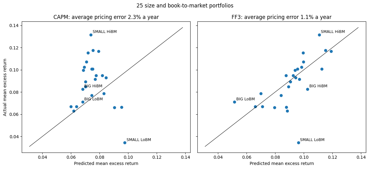
Under the CAPM, the portfolios have similar market betas, so the predicted returns bunch together while the actual returns spread out: small value stocks (SMALL HiBM) earn far more than predicted, and small growth stocks (SMALL LoBM) far less. Adding SMB and HML spreads the predictions out and pulls most points toward the line. Small growth stocks are still far below it, which is the best-known failure of the three-factor model.

Reading Fama-French as an ICAPM. Fama and French (1996) and Fama (1996) interpret the three-factor model as an ICAPM, with SMB and HML standing in for state variables that investors want to hedge. A looser reading needs no state variables: SMB and HML capture a large share of the common movement in stock returns, which a portfolio cannot diversify away. Either way, this is an interpretation, not a derivation. No one has shown which state variables SMB and HML track, and others argue the premiums come from mispricing instead of risk (Lakonishok, Shleifer, and Vishny 1994).

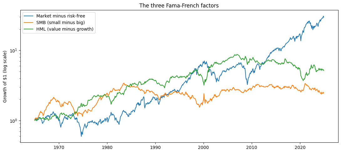
The factors have earned their premiums on average, but not smoothly. The figure shows the growth of $1 in each one.

Back to mean-variance

The story ends where it started. The CAPM says the market alone is the tangency portfolio. A multifactor model says the tangency portfolio is a mix of the factors, so Mkt, SMB, and HML together should reach a higher Sharpe ratio than the market alone, and no other portfolio should have an alpha once all three are in the regression. HW 1 Guide E tests both claims on the portfolios your HW 1 pipeline builds.

Discussion

Are SMB and HML rewards for risk, or are they mispricing? What evidence would tell the two apart?

Some answers that could come up:

• Risk predicts bad times. If the premiums compensate for risk, the factors should do badly in bad times, such as recessions or periods of low consumption, when investors can least afford losses.

• Mispricing predicts corrections. Lakonishok, Shleifer, and Vishny argue that investors extrapolate past growth and overprice growth stocks. Value stocks would then earn more as those expectations are corrected, for example around earnings announcements.

• Publication should shrink mispricing. Once a mispricing is published, traders can exploit it and it should fade. Returns on published predictors do fall after publication (McLean and Pontiff 2016). HML’s weak run since the late 2000s, visible in the figure above, is consistent with this, though it is also consistent with bad luck.

• Data mining. Hundreds of candidate factors have been proposed, and some will look priced by chance alone (Harvey, Liu, and Zhu 2016).

• Name the state variable. The ICAPM reading is testable only if SMB and HML predict changes in investment opportunities, such as future market returns or economic growth.

References

• Breeden, Douglas T. “An Intertemporal Asset Pricing Model with Stochastic Consumption and Investment Opportunities.” Journal of Financial Economics 7, no. 3 (1979): 265-296.

• Fama, Eugene F. “Multifactor Portfolio Efficiency and Multifactor Asset Pricing.” Journal of Financial and Quantitative Analysis 31, no. 4 (1996): 441-465.

• Fama, Eugene F., and Kenneth R. French. “Common Risk Factors in the Returns on Stocks and Bonds.” Journal of Financial Economics 33, no. 1 (1993): 3-56.

• Fama, Eugene F., and Kenneth R. French. “Multifactor Explanations of Asset Pricing Anomalies.” Journal of Finance 51, no. 1 (1996): 55-84.

• Harvey, Campbell R., Yan Liu, and Heqing Zhu. “… and the Cross-Section of Expected Returns.” Review of Financial Studies 29, no. 1 (2016): 5-68.

• Lakonishok, Josef, Andrei Shleifer, and Robert W. Vishny. “Contrarian Investment, Extrapolation, and Risk.” Journal of Finance 49, no. 5 (1994): 1541-1578.

• McLean, R. David, and Jeffrey Pontiff. “Does Academic Research Destroy Stock Return Predictability?” Journal of Finance 71, no. 1 (2016): 5-32.

• Merton, Robert C. “An Intertemporal Capital Asset Pricing Model.” Econometrica 41, no. 5 (1973): 867-887.

• Merton, Robert C. Continuous-Time Finance. Revised edition. Cambridge, MA: Blackwell, 1992.